Quickstart

Obtaining statistics

In order to obtain statistics from coalescent distributions, we first need to define such a distribution. This is done by creating a Coalescent object which serves as an entry point from which all statistics can be obtained. Below is an example of a simple Kingman coalescent distribution with n=10 lineages, and a single population of constant size 1.

library(phasegen)

pg <- load_phasegen()

coal <- pg$Coalescent(
    n = 10,
    demography = pg$Demography(
        pop_sizes = 1
    )
)

We can now access various statistics from this distribution which are made available as cached properties of the component distribution of the Coalescent object:

# mean coalescence time or tree height
coal$tree_height$mean

1.8

# variance of the coalescence time
coal$tree_height$var

1.15814184933233

# expected total branch length
coal$total_branch_length$mean

5.65793650793651

# expected site-frequency spectrum
barplot(coal$sfs$mean$data, main = "SFS")

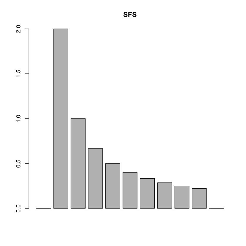
In fact, coal.tree_height, coal.total_branch_length, and coal.sfs are all PhaseTypeDistribution objects which can be accessed to obtain statistics on these distributions. If you would like to take a closer look at the API reference, these are TreeHeightDistribution, PhaseTypeDistribution, and UnfoldedSFSDistribution, respectively. PhaseTypeDistribution instances support the computation of moments and cross-moments of arbitrary order, which is only limited by the computational burden associated with higher-order moments. TreeHeightDistribution extends PhaseTypeDistribution and offers additional information through the PDF, CDF and quantile function.

coal$tree_height$quantile(0.95)

3.89324951171875

x <- seq(0, 4, length.out = 100)

plot(x, coal$tree_height$pdf(x), type = "l", main = "PDF")

Before we discuss on how to obtain more complex statistics, let us first define a more complex coalescent distribution. Here, we define a two-population coalescent using the BetaCoalescent model, where the population sizes and migration rates are time-dependent. This is done by specifying a Demography object, which is configured with a series of DemographicEvent objects.

coal <- pg$Coalescent(
    n = pg$LineageConfig(list(pop_0 = 3, pop_1 = 5)),
    model = pg$BetaCoalescent(alpha = 1.7),
    demography = pg$Demography(c(
        pg$PopSizeChange(pop = "pop_0", time = 0, size = 1),
        pg$PopSizeChange(pop = "pop_1", time = 0, size = 1.2),
        pg$PopSizeChange(pop = "pop_1", time = 5, size = 0.1),
        pg$PopSizeChange(pop = "pop_1", time = 5.5, size = 0.8),
        pg$MigrationRateChange(source = "pop_0", dest = "pop_1", time = 0, rate = 0.2),
        pg$MigrationRateChange(source = "pop_0", dest = "pop_1", time = 8, rate = 0.3),
        pg$MigrationRateChange(source = "pop_1", dest = "pop_0", time = 0, rate = 0.5)
    ))
)

We can iterate through the epochs of this demography. Within each Epoch, all rates are constant. pop_1 experiences a bottleneck at time 5, and that there is continuous migration between the two populations.

for (epoch in reticulate::iterate(coal$demography$epochs)) {
    print(epoch$to_string())
}

[1] "Epoch(start_time=0, end_time=5, pop_sizes=(pop_0=1, pop_1=1.2), migration_rates=(pop_0->pop_0=0, pop_0->pop_1=0.2, pop_1->pop_0=0.5, pop_1->pop_1=0)"
[1] "Epoch(start_time=5, end_time=5.5, pop_sizes=(pop_0=1, pop_1=0.1), migration_rates=(pop_0->pop_0=0, pop_0->pop_1=0.2, pop_1->pop_0=0.5, pop_1->pop_1=0)"
[1] "Epoch(start_time=5.5, end_time=8, pop_sizes=(pop_0=1, pop_1=0.8), migration_rates=(pop_0->pop_0=0, pop_0->pop_1=0.2, pop_1->pop_0=0.5, pop_1->pop_1=0)"
[1] "Epoch(start_time=8, end_time=inf, pop_sizes=(pop_0=1, pop_1=0.8), migration_rates=(pop_0->pop_0=0, pop_0->pop_1=0.3, pop_1->pop_0=0.5, pop_1->pop_1=0)"

Let’s take a look at the density of the underlying TreeHeightDistribution.

x <- seq(0, coal$tree_height$quantile(0.95), length.out = 100)

plot(x, coal$tree_height$pdf(x), type = "l", main = "PDF");

We can also compute higher-order moments of the SFS, such as the branch length correlation between branches subtending different numbers of lineages in the coalescent tree.

coal$sfs$corr$data

A matrix: 9 × 9 of type dbl

0	0.00000000	0.00000000	0.0000000	0.00000000	0.0000000	0.00000000	0.00000000	0
0	1.00000000	-0.03204526	-0.1390162	-0.02137022	-0.1400063	-0.01838510	0.72560160	0
0	-0.03204526	1.00000000	-0.1370290	-0.10913252	-0.1264120	0.80364349	-0.13043509	0
0	-0.13901618	-0.13702900	1.0000000	-0.15851912	0.8517271	-0.21133268	-0.16912080	0
0	-0.02137022	-0.10913252	-0.1585191	1.00000000	-0.2324032	-0.13282842	-0.09281145	0
0	-0.14000628	-0.12641201	0.8517271	-0.23240321	1.0000000	-0.19100357	-0.15794423	0
0	-0.01838510	0.80364349	-0.2113327	-0.13282842	-0.1910036	1.00000000	-0.08907693	0
0	0.72560160	-0.13043509	-0.1691208	-0.09281145	-0.1579442	-0.08907693	1.00000000	0
0	0.00000000	0.00000000	0.0000000	0.00000000	0.0000000	0.00000000	0.00000000	0

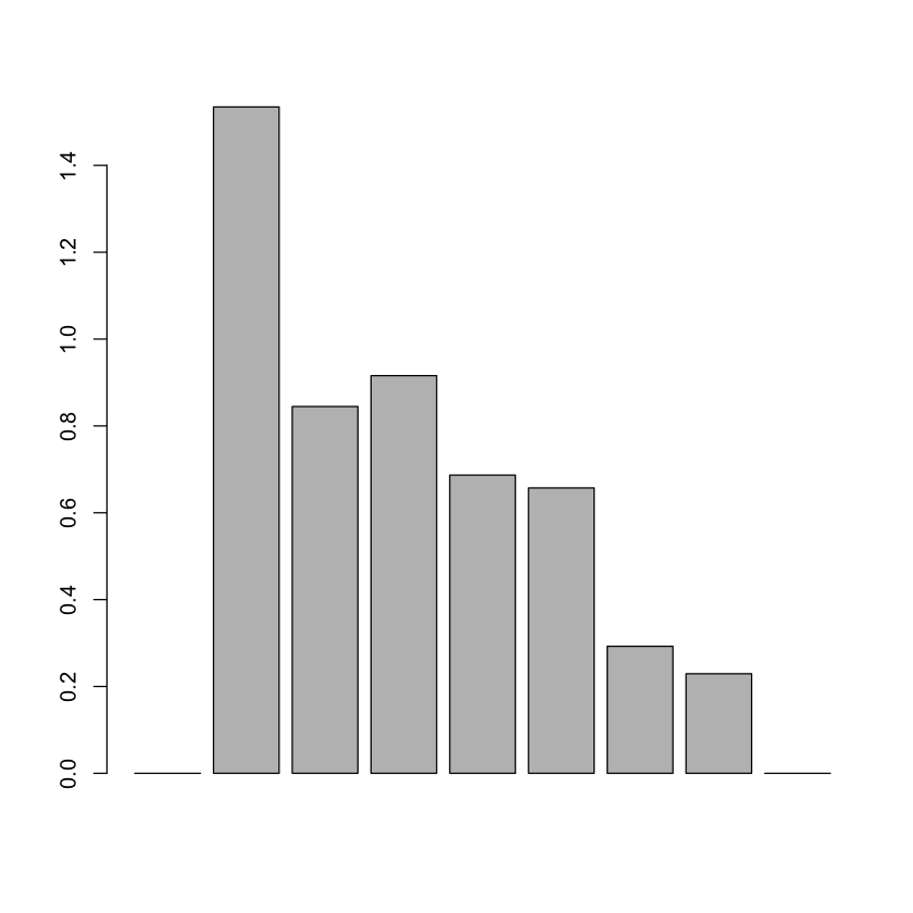
We may also marginalize over a single population. Here we obtain the mean SFS of pop_0, which represents the branch lengths for lineages that subtends i lineages in the coalescent tree, while spending time in population pop_0.

barplot(coal$sfs$demes$demes$pop_0$mean$data)

In the Using rewards section, you can read more about how to obtain more complex moments by means of specifying rewards.

Inferring parameters

The availability of exact moments lends itself to gradient-based parameter estimation. This is commonly done based on the SFS, but higher-order moments are also thinkable, provided they can be computed from the data at hand. phasegen provides a lightweight framework for performing parameter inference which is done by defining an Inference object. Inference requires a parametrized coalescent distribution, a loss function, and parameter bounds to be specified. More specifically, the coal argument is a callable that returns a Coalescent object, based on the parameter values of the current optimization step, and loss is a callable specifying the current loss. By default, 10 independent optimization runs are performed using the L-BFGS-B algorithm, and the best result is returned.

Below we optimize a one-epoch demography with a single population size change where the time of change (t) as well as the resulting population size (Ne) are variable. The observed summary statistics is an SFS with a sample size of 10, and the loss function is the Poisson likelihood.

Warning

Parallelization across multiple cores does not work when using the R interface (hence parallelize = FALSE). This is due to problems when pickling in Python the R callback specified to Inference. Problems will also arise when using to_file() and from_file().

observation = pg$SFS(
    c(177130, 997, 441, 228, 156, 117, 114, 83, 105, 109, 652)
)

inf = pg$Inference(
    bounds = list(t = c(0, 4), Ne = c(0.1, 1)),
    coal = function(t, Ne) {
        return(pg$Coalescent(
            n = 10,
            demography = pg$Demography(c(
                pg$PopSizeChange(pop = 'pop_0', time = 0, size = 1),
                pg$PopSizeChange(pop = 'pop_0', time = t, size = Ne)
            ))
        ))
    },
    loss = function(coal, x) {
        return(pg$PoissonLikelihood()$compute(
            observed = observation$normalize()$polymorphic,
            modelled = coal$sfs$mean$normalize()$polymorphic
        ))
    },
    parallelize = FALSE
)

Upon construction, the inference object is ready to be optimized and the result can be obtained.

inf$run()

for (epoch in reticulate::iterate(inf$dist_inferred$demography$epochs)) {
    print(epoch$to_string())
}

[1] "Epoch(start_time=0, end_time=0.1455, pop_sizes=(pop_0=1)"
[1] "Epoch(start_time=0.1455, end_time=inf, pop_sizes=(pop_0=0.4814)"

We may also wish to perform parametric bootstrapping. In order to do this, we provide a callback function to resample the data, and set do_bootstrap = TRUE. Note that we specify observation to Inference, which is necessary for the resampling to work. Bootstrapping can be parallelized by running multiple optimization runs independently and adding params_inferred using add_bootstrap().

Note

Note that we explicitly generate random seeds for the resampling function. This is to avoid random number generation issues when running the code through reticulate.

inf = pg$Inference(
    bounds = list(t = c(0, 4), Ne = c(0.1, 1)),
    observation = pg$SFS(
        c(177130, 997, 441, 228, 156, 117, 114, 83, 105, 109, 652)
    ),
    coal = function(t, Ne) {
        return(pg$Coalescent(
            n = 10,
            demography = pg$Demography(c(
                pg$PopSizeChange(pop = 'pop_0', time = 0, size = 1),
                pg$PopSizeChange(pop = 'pop_0', time = t, size = Ne)
            ))
        ))
    },
    loss = function(coal, observation) {
        return(pg$PoissonLikelihood()$compute(
            observed = observation$normalize()$polymorphic,
            modelled = coal$sfs$mean$normalize()$polymorphic
        ))
    },
    resample = function(sfs, x) {
        return(sfs$resample(as.integer(sample(1:1e6, 1))))
    },
    do_bootstrap = TRUE,
    parallelize = FALSE
)

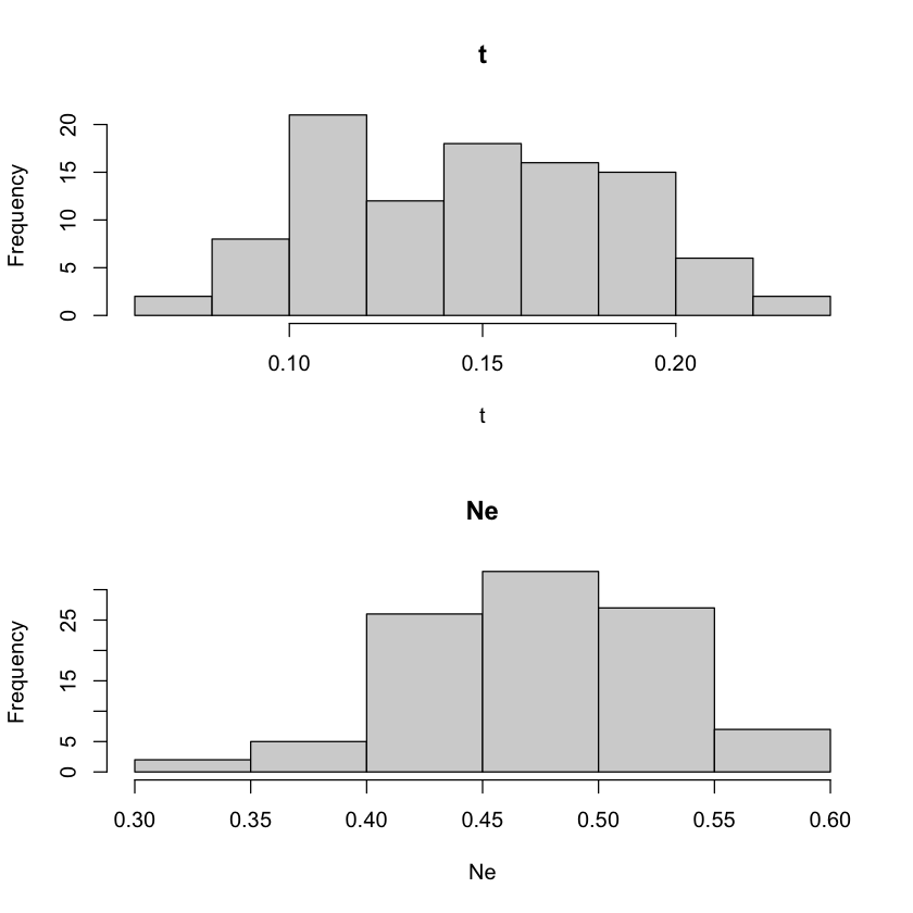
Let’s run the inference again and visualize the results.

inf$run()

par(mfrow = c(2, 1))
hist(inf$bootstraps$t, xlab = 't', main = 't')
hist(inf$bootstraps$Ne, xlab = 'Ne', main = 'Ne')