Spectra & summary statistics

Beyond scalar moments, the Coalescent provides full spectra — the joint (multi-population) and two-locus site-frequency spectra — as well as a set of standard scalar summary statistics. All of these are exact and respect the full demography and coalescent model. See Configuring the coalescent for how to configure the underlying model.

import phasegen as pg

Joint site-frequency spectrum

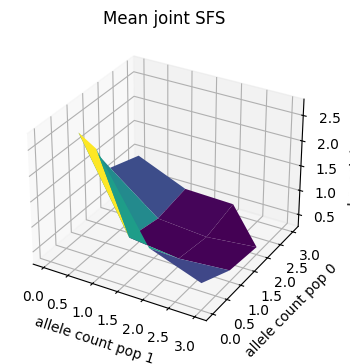
For multiple populations, jsfs() gives the joint (multi-population) SFS: the expected branch length subtending each configuration of derived-allele counts per population (the deme of origin). For P populations it is a P-dimensional JointSFS of shape (n_0 + 1, ..., n_{P-1} + 1), with higher moments available via moment(k), var and cov. It is restricted to a single locus, and the state space grows quickly with the per-population sample sizes, so keep these small.

# a two-population demography with a population-size change and asymmetric migration
coal = pg.Coalescent(
    n={'pop_0': 3, 'pop_1': 3},
    demography=pg.Demography(
        pop_sizes={'pop_0': {0: 1, 1: 0.3}, 'pop_1': {0: 1.5}},
        migration_rates={('pop_0', 'pop_1'): 0.5, ('pop_1', 'pop_0'): 0.2},
    ),
)

# mean joint SFS: expected branch length subtending each (pop_0, pop_1) allele-frequency configuration
coal.jsfs.mean.plot_surface(title='Mean joint SFS');

Two-locus SFS under recombination

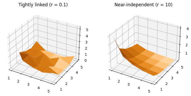
For two loci separated by recombination rate r, sfs2() gives the two-locus SFS: entry (i, j) is the expected product of the branch length subtending i samples at locus 0 and j samples at locus 1. It is a TwoLocusSFS and interpolates between the within-tree SFS covariance at r = 0 (fully linked) and independent loci as r → ∞ (for the standard coalescent). The starting linkage is set via the LocusConfig n_unlinked. A single population is supported, and the state space grows quickly with the sample size.

The single- and two-locus spectra guard each other: sfs2() requires exactly two loci, while the single-locus sfs() requires one (its marginal mean is recombination-invariant, so to obtain it for one locus simply drop the other).

# the two-locus SFS interpolates between tightly linked and independent loci as r grows
_, axs = plt.subplots(ncols=2, figsize=(9, 4), subplot_kw={"projection": "3d"})

# r = 0.1: tightly linked -> strong cross-locus structure (close to the within-tree SFS covariance)
pg.Coalescent(n=6, loci=2, recombination_rate=0.1).sfs2.mean.plot_surface(
    ax=axs[0], show=False, title='Tightly linked (r = 0.1)')

# r = 10: nearly independent -> approaches the outer product of the marginal SFS
pg.Coalescent(n=6, loci=2, recombination_rate=10.0).sfs2.mean.plot_surface(
    ax=axs[1], title='Near-independent (r = 10)');

Summary statistics

Beyond full spectra, several standard scalar summaries are available directly from the Coalescent, each respecting the full demography and coalescent model:

• Population structure — Hudson’s fst() and Patterson’s f-statistics (f2(), f3(), f4()), all derived from inter-population pairwise coalescence times.

• Linkage — the correlation of coalescence times between two loci (tree_height.loci.get_corr), which decays towards zero as the recombination rate grows.

• SFS skew — Tajima’s tajimas_d(), together with the underlying theta_pi() and theta_w() estimators.

We illustrate them on a relatively complex scenario: a structured three-population demography with asymmetric population sizes and migration.

# a structured three-population demography with asymmetric sizes and migration
struct = pg.Coalescent(
    n={'pop_0': 2, 'pop_1': 2, 'pop_2': 2},
    demography=pg.Demography(
        pop_sizes={'pop_0': 1.0, 'pop_1': 1.0, 'pop_2': 1.5},
        migration_rates={
            ('pop_0', 'pop_1'): 0.5, ('pop_1', 'pop_0'): 0.5,
            ('pop_1', 'pop_2'): 0.2, ('pop_2', 'pop_1'): 0.2,
            ('pop_0', 'pop_2'): 0.2, ('pop_2', 'pop_0'): 0.2,
        },
    ),
)

# population structure: Hudson's F_ST and Patterson's f-statistics
print(f"F_ST                    = {struct.fst:.3f}")
print(f"f2(pop_0, pop_2)        = {struct.f2('pop_0', 'pop_2'):.3f}")
print(f"f3(pop_1; pop_0, pop_2) = {struct.f3('pop_1', 'pop_0', 'pop_2'):.3f}")

F_ST                    = 0.348
f2(pop_0, pop_2)        = 4.097
f3(pop_1; pop_0, pop_2) = 1.361

# linkage: correlation of coalescence times between two loci, decaying with recombination
for r in [0.1, 1.0, 10.0]:
    corr = pg.Coalescent(n=2, loci=2, recombination_rate=r).tree_height.loci.get_corr(0, 1)
    print(f"corr(T_A, T_B) at r={r:<4} = {corr:.3f}")

corr(T_A, T_B) at r=0.1  = 0.882
corr(T_A, T_B) at r=1.0  = 0.417
corr(T_A, T_B) at r=10.0 = 0.056

# SFS skew: Tajima's D under recent population growth (excess of low-frequency variants -> D < 0)
growth = pg.Coalescent(n=10, demography=pg.Demography(pop_sizes={'pop_0': {0: 1.0, 0.5: 0.1}}))
print(f"Tajima's D (growth) = {growth.sfs.tajimas_d:.3f}")

Tajima's D (growth) = -1.263